

 By Shivali Bhadaniya
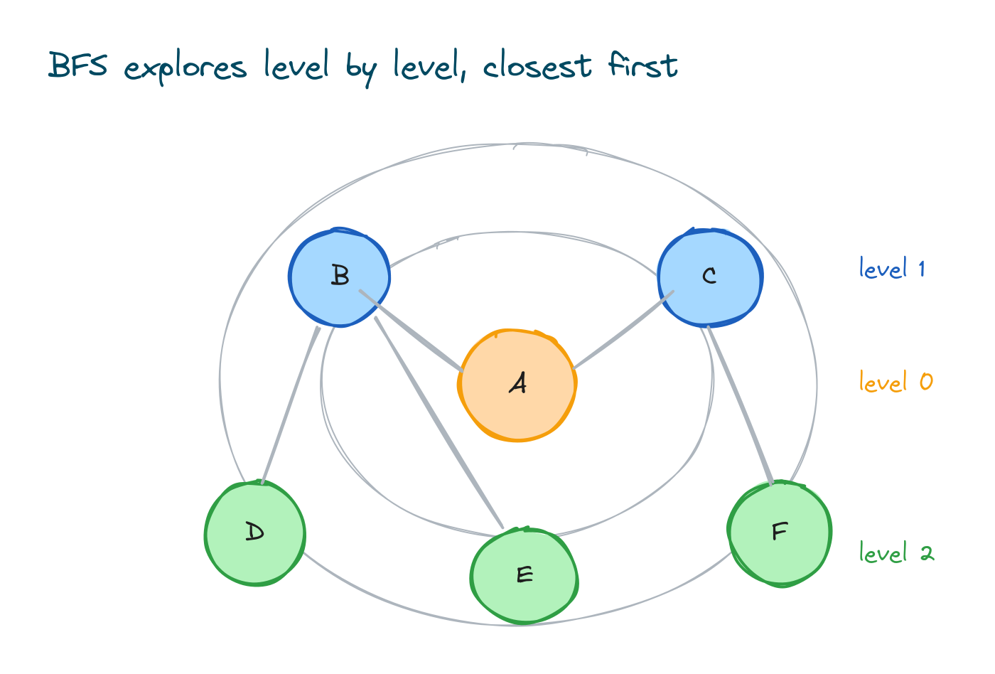
In Python, breadth first search (BFS) is a graph traversal algorithm that visits every node reachable from a starting node, in order of distance from that start. It explores all nodes one step away, then all nodes two steps away, and continues level by level until nothing is left to visit.
BFS is mainly used for three tasks: finding the shortest path in an unweighted graph, traversing a graph or tree level by level, and checking which nodes are reachable from a starting point.
What Is Breadth First Search?
Breadth first search is an algorithm that explores a graph level by level from a starting node, using a queue and a visited set. The queue holds discovered nodes waiting to be explored, first in, first out. The visited set prevents processing the same node twice. In Python, the queue is a collections.deque and the graph is usually a dictionary of lists:
from collections import deque

# 1. A graph stored as an adjacency list
graph = {"A": ["B", "C"], "B": ["A"], "C": ["A"]}

# 2. BFS visits A first, then its neighbours
queue = deque(["A"])
visited = {"A"}
order = []
while queue:
    node = queue.popleft()
    order.append(node)
    for neighbour in graph[node]:
        if neighbour not in visited:
            visited.add(neighbour)
            queue.append(neighbour)

print(order)  # Outputs: ['A', 'B', 'C']
Because BFS reaches every node by the smallest possible number of steps, it finds shortest paths in graphs where every edge counts the same.
How to Implement BFS in Python
1) Representing a Graph in Python
Before you can search a graph, you need to store it. The standard structure is an adjacency list: a dictionary where each key is a node and its value is the list of nodes it connects to. The examples in this lesson use a graph with six nodes named A through F:
graph = {
    "A": ["B", "C"],
    "B": ["A", "D", "E"],
    "C": ["A", "F"],
    "D": ["B"],
    "E": ["B", "F"],
    "F": ["C", "E"],
}

print(graph["B"])  # Outputs: ['A', 'D', 'E']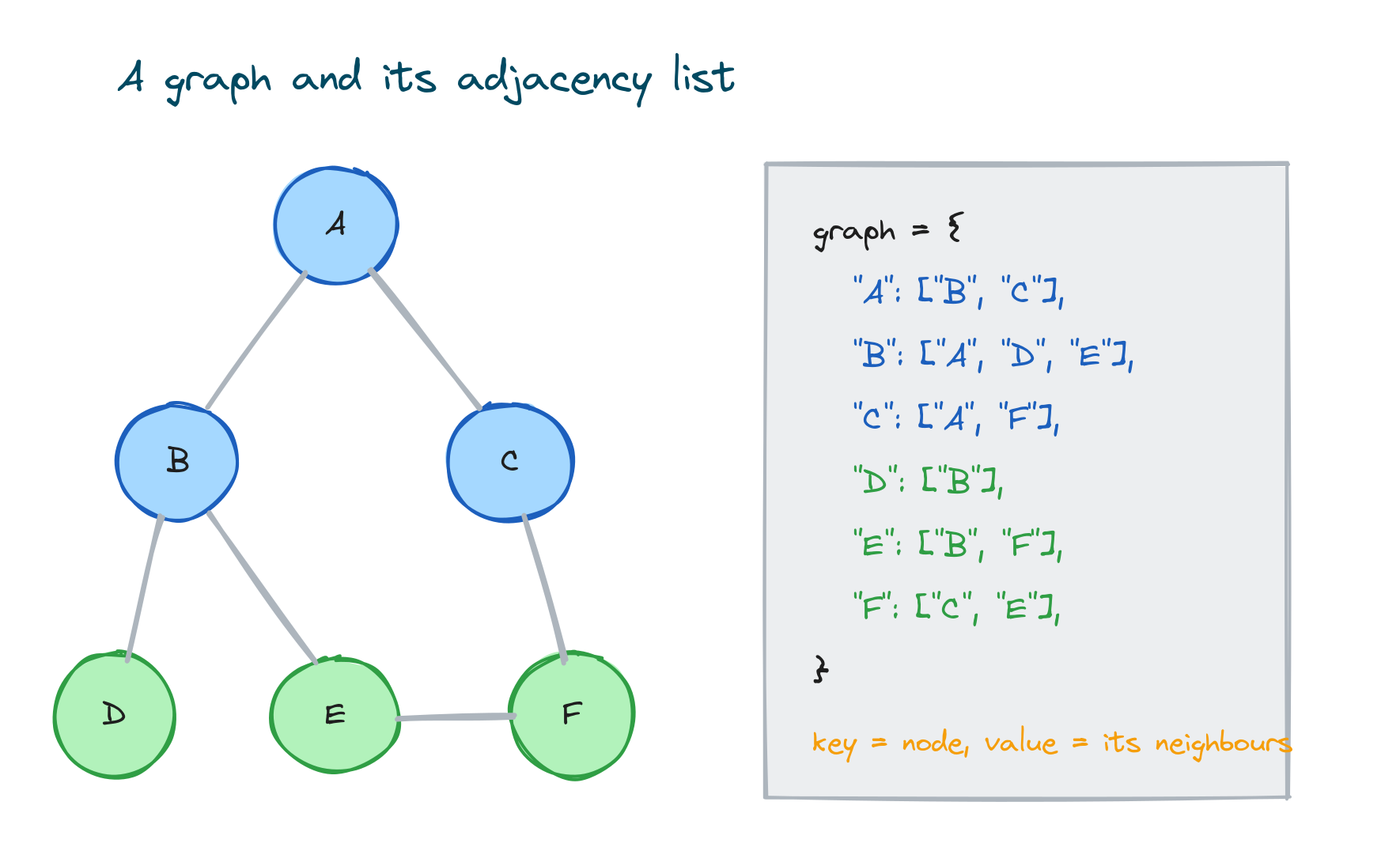
This graph is undirected, so if A connects to B, then B also lists A. In a directed graph, such as web pages linking to each other, you would list only the direction that exists.
2) The Queue and the Visited Set
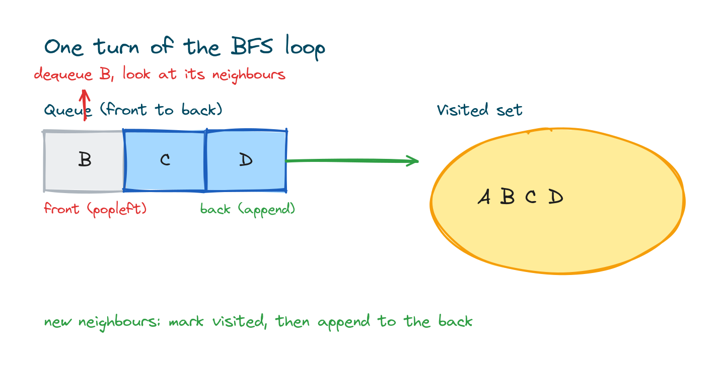
BFS relies on two data structures. The queue holds nodes that have been discovered but not yet explored. It works first in, first out, so the node added earliest is processed first, which keeps closer nodes ahead of farther ones. The stacks and queues lesson covers this structure in detail.
The visited set records every node that has been seen. Graphs can contain cycles, and without a visited set, BFS on the graph above would bounce between A and B forever.
3) Why Use collections.deque Instead of a List
A plain list can act as a queue by calling pop(0) to take the front item, but each call forces Python to shift every remaining item one position left, which takes O(n) time. Repeated for every node, the queue operations alone approach O(n²).
collections.deque, a double ended queue, adds to the back and removes from the front in O(1) constant time:
from collections import deque

q = deque(["A", "B", "C"])
q.append("D")        # add to the back, O(1)
front = q.popleft()  # remove from the front, O(1)

print(front)  # Outputs: A
print(q)      # Outputs: deque(['B', 'C', 'D'])
For a small graph the difference is invisible. For a large one, deque is the difference between fast and slow, so it is the standard choice for a BFS queue.
4) BFS Implementation in Python
The full implementation takes a node off the front of the queue, records it, and adds each unseen neighbour to the back:
from collections import deque

def bfs(graph, start):
    visited = set()
    queue = deque([start])
    visited.add(start)
    order = []

    while queue:
        node = queue.popleft()
        order.append(node)
        for neighbour in graph[node]:
            if neighbour not in visited:
                visited.add(neighbour)
                queue.append(neighbour)

    return order

graph = {
    "A": ["B", "C"],
    "B": ["A", "D", "E"],
    "C": ["A", "F"],
    "D": ["B"],
    "E": ["B", "F"],
    "F": ["C", "E"],
}

print(bfs(graph, "A"))  # Outputs: ['A', 'B', 'C', 'D', 'E', 'F']
One detail matters here: a node is marked visited when it enters the queue, not when it leaves. If marking waits until the node is dequeued, several neighbours can add the same node to the queue before it is processed.
5) BFS Example Step by Step
The table below traces the run of bfs(graph, "A"). Each row shows one turn of the loop: the node pulled off the front, the new neighbours pushed to the back, and both structures after the turn:
| Step | Dequeued | Added | Queue after | Visited after |
|---|---|---|---|---|
| 1 | A | B, C | [B, C] | A, B, C |
| 2 | B | D, E | [C, D, E] | A, B, C, D, E |
| 3 | C | F | [D, E, F] | A, B, C, D, E, F |
| 4 | D | none | [E, F] | A, B, C, D, E, F |
| 5 | E | none | [F] | A, B, C, D, E, F |
| 6 | F | none | [] | A, B, C, D, E, F |
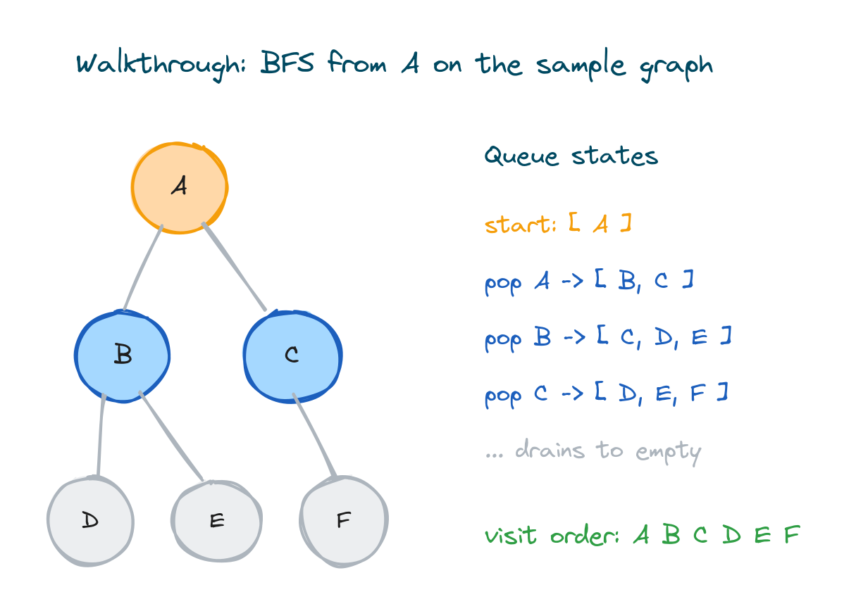
The visit order is A, then A's neighbours B and C, then their new neighbours D, E, and F. The queue grows while there is new ground to cover and drains once every node has been seen.
When to Use BFS
1) Finding the Shortest Path in an Unweighted Graph
On an unweighted graph, the first time BFS reaches a node, it has reached it by the shortest possible route, because all nodes one step away are checked before any node two steps away. To recover the actual path, a parent dictionary records which node each node was discovered from. Walking the parents backward from the target and reversing the result gives the path:
from collections import deque

def shortest_path(graph, start, target):
    if start == target:
        return [start]
    visited = {start}
    parent = {start: None}
    queue = deque([start])

    while queue:
        node = queue.popleft()
        for neighbour in graph[node]:
            if neighbour not in visited:
                visited.add(neighbour)
                parent[neighbour] = node
                if neighbour == target:
                    path = [target]
                    while parent[path[-1]] is not None:
                        path.append(parent[path[-1]])
                    return path[::-1]
                queue.append(neighbour)
    return None  # target not reachable

graph = {
    "A": ["B", "C"],
    "B": ["A", "D", "E"],
    "C": ["A", "F"],
    "D": ["B"],
    "E": ["B", "F"],
    "F": ["C", "E"],
}

print(shortest_path(graph, "A", "F"))  # Outputs: ['A', 'C', 'F']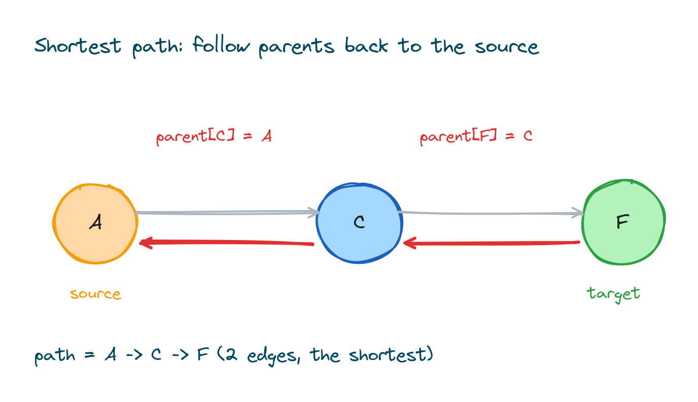
The number of edges on the path is len(path) - 1. This works only when every edge counts as one step. When edges have different weights, Dijkstra's algorithm is the correct tool instead.
2) Level Order Traversal of a Tree
A tree is a graph with no cycles, so BFS on a tree is called level order traversal. To group nodes by level, check the queue length at the start of each round: that count is exactly one full level.
from collections import deque

tree = {
    1: [2, 3],
    2: [4, 5],
    3: [6, 7],
    4: [], 5: [], 6: [], 7: [],
}

def level_order(tree, root):
    levels = []
    queue = deque([root])
    while queue:
        level_size = len(queue)
        current = []
        for _ in range(level_size):
            node = queue.popleft()
            current.append(node)
            for child in tree[node]:
                queue.append(child)
        levels.append(current)
    return levels

print(level_order(tree, 1))  # Outputs: [[1], [2, 3], [4, 5, 6, 7]]
No visited set is needed on a tree, because a tree has no cycles. On a general graph the set is still required.
3) Traversing a Disconnected Graph
BFS from one start only reaches nodes connected to that start. If the graph has separate components, an outer loop over every vertex starts a fresh BFS from any node that has not been visited yet. Each fresh start finds one connected component:
from collections import deque

graph = {
    "A": ["B"],
    "B": ["A", "C"],
    "C": ["B"],
    "X": ["Y"],
    "Y": ["X"],
}

def bfs_from(graph, start, visited):
    order = []
    queue = deque([start])
    visited.add(start)
    while queue:
        node = queue.popleft()
        order.append(node)
        for neighbour in graph[node]:
            if neighbour not in visited:
                visited.add(neighbour)
                queue.append(neighbour)
    return order

def bfs_all(graph):
    visited = set()
    components = []
    for node in graph:
        if node not in visited:
            components.append(bfs_from(graph, node, visited))
    return components

print(bfs_all(graph))  # Outputs: [['A', 'B', 'C'], ['X', 'Y']]
BFS vs DFS in Python
BFS and DFS visit the same nodes in a different order. BFS uses a queue and spreads out level by level. DFS uses a stack, often the call stack through recursion, and follows one branch to its end before backing up:
| BFS | DFS | |
|---|---|---|
| Data structure | Queue (deque) | Stack or recursion |
| Order | Level by level, closest first | One deep branch at a time |
| Shortest path (unweighted) | Yes, found directly | Not guaranteed |
| Memory | Can hold a whole level at once | Holds one path at a time |
| Typical uses | Nearest node, shortest hops, level order | Cycle detection, topological sort, path existence |
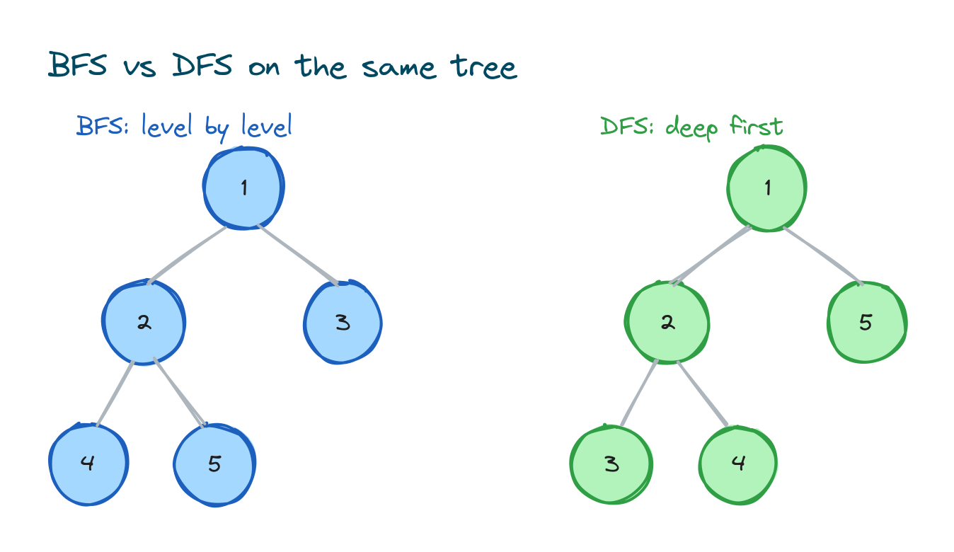
BFS suits questions about distance or the fewest steps. DFS suits questions about structure, such as whether a path or cycle exists.
Examples of Using BFS in Python
1) Finding the Distance to Every Node
Storing a step count instead of a parent gives the distance from the start to every reachable node:
from collections import deque

def distances(graph, start):
    dist = {start: 0}
    queue = deque([start])
    while queue:
        node = queue.popleft()
        for neighbour in graph[node]:
            if neighbour not in dist:
                dist[neighbour] = dist[node] + 1
                queue.append(neighbour)
    return dist

graph = {"A": ["B", "C"], "B": ["A", "D"], "C": ["A"], "D": ["B"]}
print(distances(graph, "A"))
# Outputs: {'A': 0, 'B': 1, 'C': 1, 'D': 2}
2) Checking if a Path Exists
Returning as soon as the target appears answers reachability questions without exploring the rest of the graph:
from collections import deque

def can_reach(graph, start, target):
    visited = {start}
    queue = deque([start])
    while queue:
        node = queue.popleft()
        if node == target:
            return True
        for neighbour in graph[node]:
            if neighbour not in visited:
                visited.add(neighbour)
                queue.append(neighbour)
    return False

graph = {"A": ["B"], "B": ["A", "C"], "C": ["B"], "X": ["Y"], "Y": ["X"]}
print(can_reach(graph, "A", "C"))  # Outputs: True
print(can_reach(graph, "A", "X"))  # Outputs: False
Learn More About Breadth First Search
Time and Space Complexity of BFS
BFS visits each vertex once and examines each edge once, so the time complexity is O(V + E), where V is the number of vertices and E the number of edges. This assumes an O(1) queue, which is why deque matters; a list-based queue adds an extra factor on top.
The space complexity is O(V). In the worst case the queue and the visited set each hold every vertex. On a wide graph the queue can contain an entire level at once, which is why BFS can use more memory than DFS.
Applications of BFS
BFS appears wherever the question involves the closest match or the fewest steps:
- Shortest path in a maze or grid - where every move costs the same.
- Social networks - measuring degrees of separation between two people.
- Web crawlers - visiting pages layer by layer out from a seed page.
- Routing and broadcasting - working out how far a message spreads in each hop.
- Weighted variants - as the base idea behind Dijkstra's algorithm.
Graph traversal is also a staple of coding interviews, so it is worth being able to explain a BFS solution step by step.
Key Takeaways for BFS
- Level by level - BFS explores a graph outward from a start node, closest nodes first, using a queue and a visited set.
- Use
collections.deque- Itspopleft()is O(1), whilelist.pop(0)is O(n) because the list shifts every remaining item. - Mark visited on enqueue - Marking a node when it enters the queue prevents it from being added more than once.
- Shortest paths, unweighted only - BFS finds shortest paths when every edge counts as one step; weighted graphs need Dijkstra's algorithm.
- Disconnected graphs need an outer loop - Start a fresh BFS from every unvisited vertex to cover all components.
- Cost - O(V + E) time and O(V) space.
BFS explores level by level, and its counterpart depth first search follows one branch to its end before backtracking. The two together cover most graph problems you will meet.