Quick Sort in C++ ( Code with Example)

Sorting refers to the process of rearranging elements present in a data structure in ascending or descending order and the algorithms which achieve this task are known as sorting algorithms. The need for finding an algorithm that produces an ordered structure in minimum time and space has made sorting algorithms a hot topic in research. There are various sorting algorithms available in the market, some of the famous ones are merge sort, selection sort, counting sort, bubble sort, and quicksort. In this article, we will learn about quicksort and dive deep into its various aspects: working, algorithm, code, time, and space complexity. So, we request you to fasten your seat belts because it’s going to be an interesting ride.

What is the Quick Sort?

As the name suggests, this algorithm is quick or fast in terms of speed and this is one of the reasons why it is so famous. This algorithm is based on the divide and conquer approach of programming. If you are familiar with merge sort then you may know what is this approach is, and if not don’t worry we will explain it in brief. The divide and conquer approach involves dividing a task into small atomic sub-tasks and then solving those subtasks. The results of those subtasks are then combined and evaluated to get the final result.

Let us now discuss how this approach applies to the quick sort algorithm. In the quick sort algorithm, we select a pivot element and we position the pivot in such a manner that all the elements smaller than the pivot element are to its left and all the elements greater than the pivot are to its right. The elements to the left and right of the pivot form two separate arrays. Now the left and right subarrays are sorted using this same approach. This process continues until each subarray consists of a single element. When this situation occurs, the array is now sorted and we can merge the elements to get the required array.

Two important characteristics of the quick sort algorithm are that it is an inplace algorithm and is not stable.

How to select the pivot element?

There are 4 common ways of selecting a pivot. One can use any one of the following methods:

1. Pick the first element
2. Pick the last element
3. Pick a random element
4. Pick the median element

In this article, we will be picking the last element as the pivot.

Algorithm for Quick Sort

The quick algorithm consists of two different algorithms, one for partitioning the array according to the pivot and one for actual sorting. Let us look at both the algorithms one by one. Let us first discuss the algorithm of partitioning the array.

Step 1: Take two elements low and high

Step 2: Make low store the starting index of the array

Step 3: Make high store the last index of the array

Step 4: Take a variable j and initialize it to low

Step 5: Take pivot as the last element is the array

Step 6: Traverse through the entire array using the variable i and compare each element with pivot

Step 7: If arr[i] < pivot then increment j and swap element as position j and i

Step 8: Increment i by 1

Step 9: When the loop terminates, return j – 1

The value returned by the partitioning algorithm gives us the correct position or index of the pivot in the array. What is meant by correct position is that all elements preceding the pivot are smaller than the pivot and all the elements after the pivot are greater than it. Let us now look at the sorting algorithm.

Step 1: Take pivot as the last element in the array

Step 2: Find the correct index of the pivot using the partition algorithm

Step 3: Recursively call Quicksort on the left subarray

Step 4: Recursively call Quicksort on the right subarray

Example of quick sort

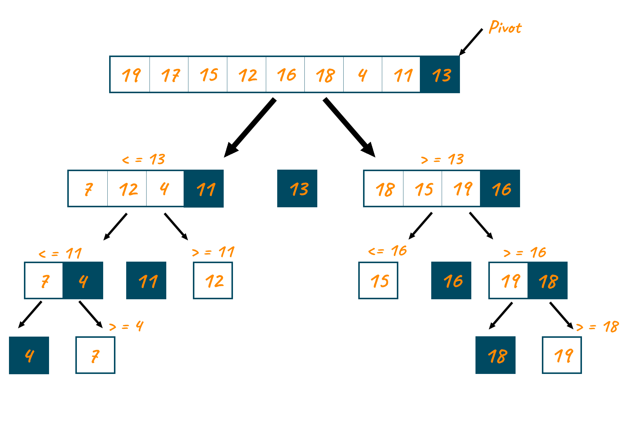
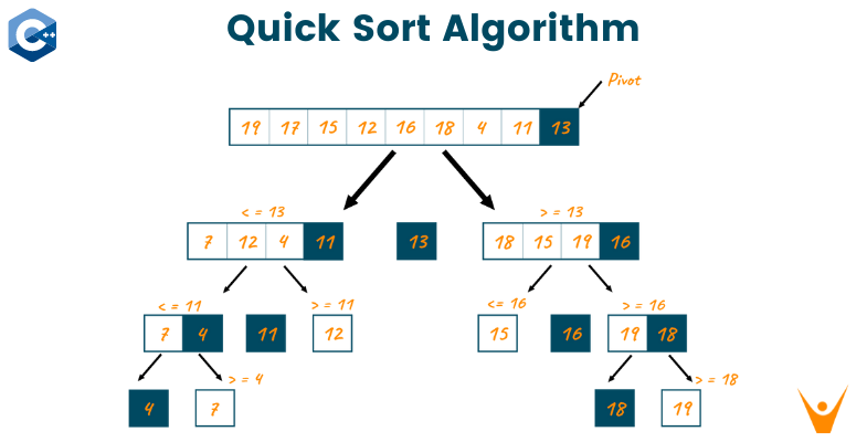
Let us now look at an example to understand the quicksort algorithm better. Imagine all the recursive calls organized in the form of a tree structure. Don't worry we are not going to use a tree data structure, but organizing the recursive calls in the form of a tree helps us in visualizing the algorithm. When the quicksort algorithm first gets called with the given array, 13 gets selected as the pivot. Positioning this pivot results in the formation of two subarrays. The quicksort algorithm now gets called on the left subarray and 11 gets selected as the pivot and it is positioned at the correct index.

The left subarray gets further divided and the quicksort algorithm gets called on the array containing elements 7,4. Here 4 gets selected as the pivot and now the array gets partitioned into parts each containing one single element.

Since an array containing a single element is already sorted, therefore, the recursive calls start returning. The right subarray containing the element 12, formed after the second partition, also contains a single element, and hence this function call returns. The left subarray containing the elements [7, 12, 4, 11] is now sorted and this same procedure repeats for the right subarray containing the elements [18, 15, 19, 16].

C++ Code for Quick Sort

The following code shows the implementation of quicksort in C++.

#include
using namespace std;

void swap(int arr[] , int pos1, int pos2){
	int temp;
	temp = arr[pos1];
	arr[pos1] = arr[pos2];
	arr[pos2] = temp;
}

int partition(int arr[], int low, int high, int pivot){
	int i = low;
	int j = low;
	while( i <= high){
		if(arr[i] > pivot){
			i++;
		}
		else{
			swap(arr,i,j);
			i++;
			j++;
		}
	}
	return j-1;
}

void quickSort(int arr[], int low, int high){
	if(low < high){
	int pivot = arr[high];
	int pos = partition(arr, low, high, pivot);
	
	quickSort(arr, low, pos-1);
	quickSort(arr, pos+1, high);
	}
}

int main()
{
	int n ;
	cout << " enter the size of array";
	cin>>n;
	int arr[n];
	for( int i = 0 ; i < n; i++){
		cin>> arr[i];
	}
	quickSort(arr, 0 , n-1);
	cout<<"The sorted array is: ";
	for( int i = 0 ; i < n; i++){
		cout<< arr[i]<<"\t";
	}
	
}

Output

enter the size of array5
32
21
54
76
45
The sorted array is: 21     32      45      54      76

Time complexity and space complexity

The running time complexity of quicksort for the best case and the average case is O(N log N). Whereas the time complexity is for the worst case is O( N2). Coming to the space complexity, since the quick sort algorithm doesn’t require any additional space other than that to store the original array, therefore, the space complexity of the quick sort algorithm is O(N). N is the size of the input array.

Applications of Quick Sort

The various fields where quicksort is used are:

• Commercial computing
• Numerical computations
• Information searching

Advantages of quicksort

• The average-case time complexity to sort an array of n elements is O(n lg n).
• Generally, it runs very fast. It is even faster than merge sort.
• No extra storage is required

Disadvantages of quicksort

• Its running time can be different for different array contents.
• The worst-case quick sort takes place when the array is already sorted. 
• It is not stable.

Conclusion

The speed of the quick sort algorithm makes it one of the most important sorting algorithms. This is why one when learning sorting algorithms shouldn’t skip over this algorithm. In this article, we visited quick sort in great detail including its implementation in C++. We recommend you to visit other sorting algorithms as well like merge sort and selection sort.