[Guide] Data Structure and Algorithms in 2021 (for Beginners)

In this article we studied, we will study the data structure and algorithm (DSA) concepts along with an introduction to them. We will go through every classification of data structure in brief. Also, we will study some algorithm techniques. This is a complete Data Structures and Algorithms guide for beginners in 2021. So, let's get started!

What is Data Structure?

A malicious program that is a collection of instruction to perform a selected task. For this, a computer program may have to store data, retrieve data, and perform computations on the data. The data structure is a specific method of organizing data in a computer so it can often be used effectively. The data structure is a named location that will be store and organize data. And, an algorithm is a collection of steps to resolve a specific problem. Learning data structures and algorithms permit us to write efficient and optimized computer programs. for instance, we will store a list of elements having a similar data type victimization the array data structure.

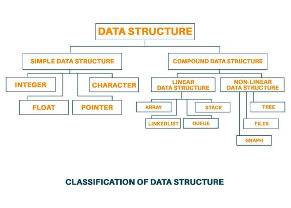
Classification of Data Structure

Data Structure is classified into two categories:

1. Simple Data Structure: These are very basic data structures that can be directly operated by machine instruction. For example Float, Integer, Character, Strings, etc
2. Compound Data Structure: Compound data structure can be constructed with the help of any one of the simple data structures and have its specific functionality. Language provides a way of defining its data type and these are called a compound data structure. These data structures are very sophisticated. The compound data structure emphasizes the structuring of a group of heterogeneous and homogenous data elements.

Classification of Compound Data Structure

Compound data structures are further divided into two categories: 1) Linear Data Structure and 2) Non-Linear Data Structure.

Linear Data Structure

A linear data structure traverses the data sequentially, in which only one data element can be directly reached. For Example Array, Linked list, Stack, Queue.

Let us study the linear data structure one by one in detail:

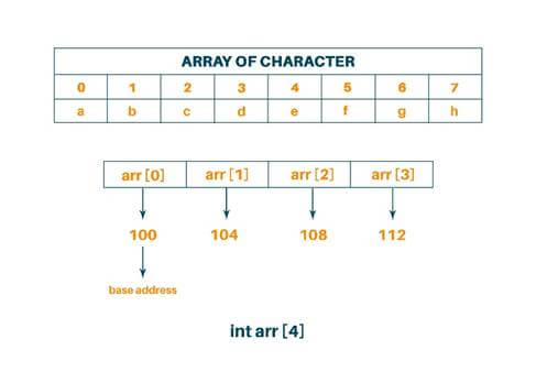
• Array: An array is a data structure that holds fix number of elements and these elements should be of the same data type. Most of the data structure makes use of an array to implement their algorithm. There is two important part of the array: 1) Element-Each item store in the array is called an element. 2) Index- Every element in the array have its numerical value to identify the element. These elements allocate contiguous memory locations that allow easy modifications in data.

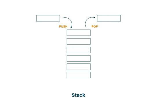
• Stack: A stack is a data structure in which items can be inserted only from one end and get items back from the same end. Then, the last item inserted into the stack is the first item to be taken out from the stack. In short, it is called Last In First Out (LIFO). We can also consider the stack as a real physical stack or pile. Stack features insertion and deletion of elements at one end called top of the stack. Three basic operations can be performed on the stack. They are push (inserting an item into stack), pop (deleting an item from the stack), pip (displaying the content of the stack).

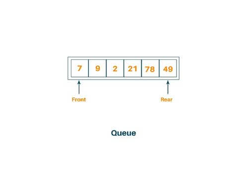
• Queue: A queue is two ended data structure in which an item can be inserted from one end and taken out from the other end. Therefore, the first item inserted in the queue is the first item to be taken out of the queue. This property is called First In First Out (FIFO). In the queue, we insert the element from the REAR end and delete the element from the FRONT end only. There are two ways to implement queue and i.e is arrays and pointers.

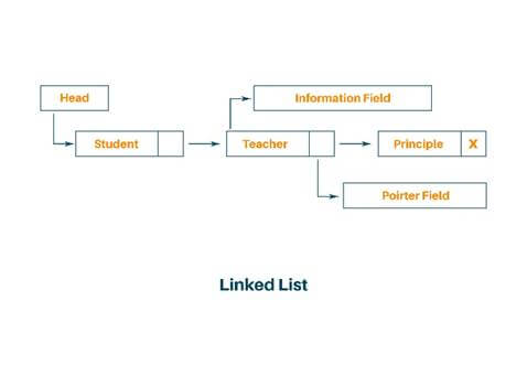
• Linked List: Linked List can be alternately used to store items. In the linked list space to store an item is created as is needed and destroyed when space is no longer required to store the item. Hence, the linked list is a dynamic data structure. Every list has two fields, 1) One field is used to store the data, and 2) Another field is used for storing the address of the next data element. Therefore, lists are a kind of container.

Non-Linear Data Structure

Every data item is attached to several other data items in a way that is specific for reflecting the relationship the data items here are not stored in the sequential structure. Example: Tree, Graph, Files, etc.

Let us study the non-linear data structure one by one:

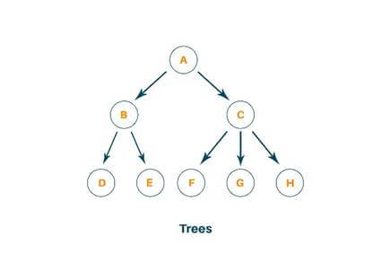
• Tree: A tree is a non-linear data structure that is mainly used to represent the data containing the hierarchical relationship between elements known as nodes. The topmost node in the hierarchy is called the root and the bottommost node in the tree is called the leaf node. Each node contains the pointers to point to its adjacent node. A tree data structure is based on the parent-child relationship among the nodes.

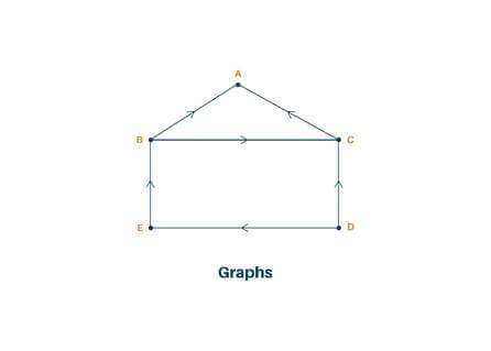
• Graph: It is the set of items connected by edges. Each item is called the vertex or node. Trees are a special kind of graph but the difference between them is that a graph can have a cycle while a tree cannot have a cycle. Graphs are usually represented by G=(V, E), V is set vertices and E is the set of edges. A graph can be known as a pictorial representation of a set of elements.

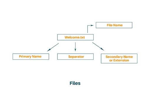
• Files: The file is the collection of records related to each other. The size of the file is limited by the size of the memory and storage medium. There are two important features of a file 1) File activity and 2) File volatility.

Concepts of Tree Data Structure

1. Binary Tree: A binary tree is a tree such that every node has at most 2 children and each node is labeled as either left or right.
2. AVL Tree: A tree is perfectly balanced if it is empty or the number of nodes in each subtree differs by not more than 1. A perfectly balanced tree is not created by the AVL tree. Instead, it creates a height-balanced tree. The height balance of the node is calculated as follows:

height balance of node = height of right subtree - the height of left subtree

A binary tree is said to be AVL balanced if 1) The difference in the height between the left and right subtree is at most 1, and 2) Both subtrees are themselves AVL tree.

B-Tree: A B-tree of order m is an m-way tree (i.e., a tree where each node may have up to m children) in which:

1. the number of keys in each non-leaf node is one less than the number of its children and these keys partition the keys in the children in the fashion of a search tree
2. all leaves are on the same level
3. all non-leaf nodes except the root have at least ém / 2ù children
4. the root is either a leaf node, or it has from two to m children
5. a leaf node contains no more than m – 1 keys

The number m should always be odd

2-3 Tree: A 2-3 tree is a tree in which each internal node(non-leaf) has either 2 or 3 children, and all leaves are at the same level. A node may contain 1 or 2 keys. All leaf nodes are at the same depth. All non-leaf nodes have either 1 key and two subtrees or 2 keys and three subtrees.

Concepts of Graph Data Structure

1. Breadth First Search: Breadth-First Search (BFS) is an algorithm used for traversing graphs or trees. Traversing means visiting each node of the graph. Breadth-First Search is a recursive algorithm to search all the vertices of a graph or a tree.BFS can be implemented by using data structures like a dictionary and lists. Breadth-First Search in tree and graph is almost the same. The only difference is that the graph may contain cycles, so we may traverse to the same node again.
2. Depth First Search: The Depth-First Search is a recursive algorithm that uses the concept of backtracking. It involves thorough searches of all the nodes by going ahead if potential, else by backtracking. Here, the word backtrack means once you are moving forward and there are no more nodes along the present path, you progress backward on an equivalent path to hunt out nodes to traverse. All the nodes are progressing to be visited on the current path until all the unvisited nodes are traversed after which subsequent paths are going to be selected.
3. Minimum Spanning Tree: A spanning tree of a graph is just a subgraph that contains all the vertices and is a tree. A graph may have many spanning trees. The Minimum Spanning Tree for a given graph is the Spanning Tree of minimum cost for that graph.
4. Kruskal’s Algorithm: This algorithm falls under the category of greedy algorithm. It starts with the lowest weight edge and keeps adding until we achieve a minimum spanning tree. Steps of applying Kruskal's algorithm:
   1. Sort all edges from low to high weight
   2. Take the edge with the lowest weight and add it to the spanning tree and if adding edges create a cycle, then reject the edge.
   3. Keep adding edge until we reach all vertices.
5. Prim’s Algorithm: This algorithm falls under the category of greedy algorithm. It starts with the lowest weight edge and keeps adding until we achieve a minimum spanning tree. Steps of applying prim’s algorithm:
   1. Choosing a vertex at random and initializing the minimum spanning tree.
   2. Find all the edges that connect the tree to new vertices, and add the minimum edge to the tree.
   3. Keep repeating the above steps until you find the minimum spanning tree.
6. Dijkstra’s Algorithm: This algorithm allows to find the shortest path between any two vertices of a graph. First, we overestimate the distance of each vertex from the starting vertex and then we visit each node and its neighbor to find the shortest subpath to those neighbors. The algorithm uses the greedy approach.

What is an Algorithm?

An algorithm is any well-defined procedure that takes some values or set of instructions as input and produces some values or set of values as output. An algorithm is a sequence of computational steps that transform the input into the corresponding output. An algorithm is a set of instructions for carrying out calculations either by hand or on a machine. It is an abstraction of a program to be executed on a physical machine.

Analysis of Algorithm

The analysis of an algorithm is the process of comparing the various algorithm to solve the same problem. Analysis of the algorithm is done to analyze which algorithm takes less time, effort, and memory to solve a particular problem.

Types of analysis of algorithm:

1. Best Case: Best case analysis we calculate the lower bound on running time of the algorithm. The best-case causes a minimum number of operations to be executed.
2. Average Case: In average case analysis we take all possible input and calculate computing time for all of the input. It lies between the best case and the worst case.
3. Worst Case: Worst-case analysis we calculate the upper bound on running time of the algorithm. The worst-case causes a maximum number of operations to be executed.

Divide and Conquer Technique

To solve a given problem, algorithms call themselves recursively one or more time to deal with closely related subproblems, therefore we can say that the algorithms are recursive in structure. These algorithms typically follow a divide-and-conquer approach:

The divide-and-conquer approach involves three steps to follow:

1. Divide: Break the problem into several subproblems that are similar to the original problem but smaller in size.
2. Conquer: Solve the subproblem recursively, and if the subproblem size is already small enough, just straightforwardly solve the problem.
3. Combine: Combine this solution to create a solution to the original problem.

Dynamic Programming

Dynamic programming solves the problem by combining the solution of the subproblem, just like the divide and conquer method. Dynamic programming is applicable when the subproblem is not independent, which means when the subproblem shares the subproblem. A dynamic programming algorithm solves every subproblem just once and then saves its answer in the table, thereby avoiding the work of recomputing the answer every time the subproblem is encountered.

The dynamic programming algorithm obtains the solution using the principle of optimality. The principle of optimality states that “in an optimal sequence of decisions or choices, each sequence must also be optimal”.

Greedy Programming

Greedy Algorithm works by making the decision that seems most promising at any given moment and it never reconsiders this decision whatever situation may arise. To solve the problem in an optimal way using the greedy approach, there is a set or list of candidate C. Once the candidate is selected in the solution, it is forever there, and if once the candidate is rejected once then it is never reconsidered. To construct the solution optimally, the Greedy algorithm maintains two sets. One set contains candidates that have already been considered and chosen, while the other set contains the candidate that has been considered but rejected. Finding the minimum spanning tree from the given graph using Kruskal’s algorithm and prim’s algorithm is done using the Greedy approach.

Conclusion

Hence, in this blog, we studied what is data structure and its detailed classification. Also, we understood what is algorithm and the different techniques of algorithm analysis. Other than this there are many concepts under data structure and algorithm. But this is always enough to start with for beginners but still if you need data structures assignment help then our experts are available 24/7.